Introduction

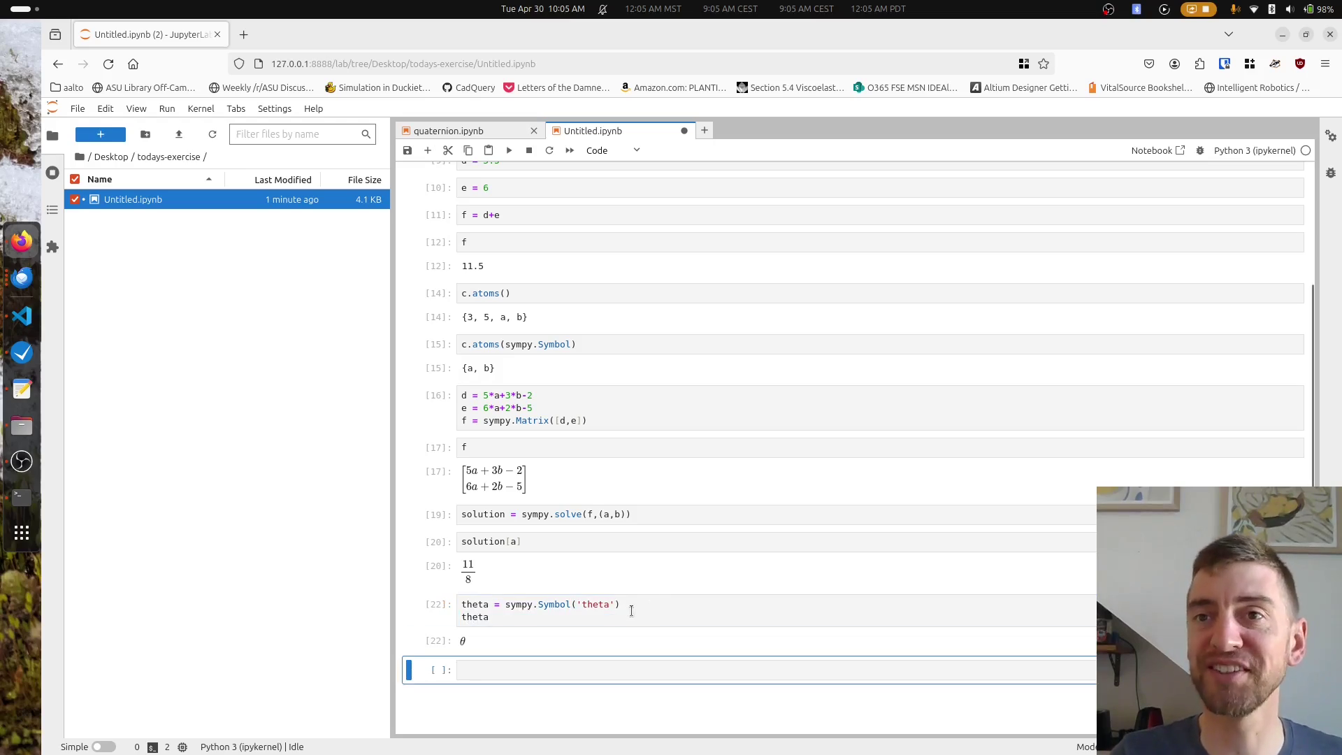
If you like keeping all your computing in one language (and that language is Python), but want some of the equation manipulation capabilities of Mathematica, have you tried Sympy?

Using Sympy in Expressions

The sympy package in Python is useful for forming and working with symbolic expressions rather than literals. A “literal”, in programming terms, is a numeric value, like 1.2. You can assign numeric, literal values to variables in Python natively, and use python expressions to find numeric answers to expressions. But what if you wanted to work with the expression or equation itself? This is where “symbolic” variables come in.

To explore this concept, first we should import the sympy package

import sympy

To create a symbol, we instantiate sympy’s Symbol() class. It requires, at minimum, a string to define how the symbol will be reendered

a = sympy.Symbol('a')
b = sympy.Symbol('b')

To see how a is rendered in IPython or Jupyter, simply call the variable you stored the symbol in:

a

$\displaystyle a$

You can see that it is rendered, whenever possible, as a latex-style expression. This also means you can create symbolic variables that use the latex math mode’s expansive set of greek symbols. For example

theta1 = sympy.Symbol('\\theta_1')
theta1

$\displaystyle \theta_{1}$

Here we have created a symbol, stored in variable theta1, that renders as the greek letter $\theta_1$.

Note that we had to use a double backslash (\\), rather than latex’s single backslash. This is due to the fact that Python strings recognize single backslash characters as a flag for writing non-printing characters such as tab and carriage return. In fact, \t renders in a Python string as a tab character. To get around this, Python strings use the double-backslash to indicate strings where a single backslash was desired.

With symbols created, we can now begin to form symbolic expressions.

c = 5*a+3*b**2
c

$\displaystyle 5 a + 3 b^{2}$

In this case, we have stored the symbolid expression $5a+3b^2$ into a Python variable, c. In contrast, if we were working with numeric literal values, the result of a python expression are stored as a numeric value as well.

d = 5.5
e = 6
f = d+e
f

11.5

type(f)

float

When working with symbolic expressions, it is sometimes useful to list all the “atomic” values being used in the expression. This helps separate the operands from the operators. The atoms() method is useful for this:

c.atoms()

{2, 3, 5, a, b}

However, what if we want to list only the symbolic variables, rather than the numeric? We can supply Symbol to atoms() to filter out the symbolic items

c.atoms(sympy.Symbol)

{a, b}

We can work with systems of equations by forming expressions or symbolic variables into matrices or vectors. Sympy Matrix() classes are useful for that, but have some differences in the assumed structure of the vectors and matrices you form:

d = 5*a+3*b-2
e = 6*a+2*b-5
f = sympy.Matrix([d,e])
f

$\displaystyle \left[\begin{matrix}5 a + 3 b - 2\\6 a + 2 b - 5\end{matrix}\right]$

In this case, we formed a 2x1, 2-dimensional matrix. Defined in this way, we can solve the system of equations all at once using sympy.solve().

solution = sympy.solve(f,(a,b))
solution

{a: 11/8, b: -13/8}

Though the answer supplied is numeric, it is important to note that these results are still in a sympy numeric format, hence the rational result rather than a decimal float.

You can also use sympy’s many tools for operating on expressions directly. Creating a well-known expression,

g = 3*a+ 4*b +7*a+16*b-32*a*b

We can see that the simplify method is a handy tool for shortening expressions, using a number of approaches under the hood.

g.simplify()

$\displaystyle - 32 a b + 10 a + 20 b$

One of those tools is the expand() method, which can be used on its own.

g = (a+b)*(a-b)
g.expand()

$\displaystyle a^{2} - b^{2}$

simplify() also applies trigonometric simplifcations when appropriate:

f = sympy.sin(theta1)**2 + sympy.cos(theta1)**2
f.simplify()

$\displaystyle 1$

g = sympy.sin(a)*sympy.cos(b) + sympy.sin(b)*sympy.cos(a)
g.simplify()

$\displaystyle \sin{\left(a + b \right)}$

g = sympy.cos(a)*sympy.cos(b) - sympy.sin(a)*sympy.sin(b) 
g.simplify()

$\displaystyle \cos{\left(a + b \right)}$

As noted above, though, care must be taken when working on matrices and arrays between numpy and sympy. There are differences in the dimensions of structures created between these two packages. For example,

import numpy

v1  = sympy.Matrix([1,2,3])
v2  = numpy.array([1,2,3])
v3 = numpy.array([[1,2,3]])

print(v1.shape,v2.shape,v3.shape)

(3, 1) (3,) (1, 3)

As you can see, sympy Matrix classes create 2-dimensional matrices with a length of 1 column when supplied by a list. Conversely, numpy arrays, when initialized, need to have the dimensions determined by the number of nested lists. Thus, converting sympy Matrix classes to numpy.array elements must be done with care, to ensure consistency.

Derivatives

You can take the partial derivative of expressions or matrices using the diff method.

h = 1*a+2*b +3*a**2 +5*b**3
h.diff(a)

$\displaystyle 6 a + 1$

w = sympy.Matrix([a,b,3])
w.diff(a)

$\displaystyle \left[\begin{matrix}1\\0\\0\end{matrix}\right]$

For nx1 matrices (vectors), the jacobian() method is also available, which finds the partial derivatives of a vector with respect to another vector of variables.

w.jacobian(sympy.Matrix([a,b]))

$\displaystyle \left[\begin{matrix}1 & 0 \\ 0 & 1 \\ 0 & 0\end{matrix}\right]$

You can substitute one thing for another using the subs() method. This is useful for evaluating an expression with numerical values

exp = (a+b).subs({a:3, b:4})
exp

$\displaystyle 7$

Keep in mind that even numerical results of sympy substitutions are sympy numbers and need to be converted to a different data type of a given precision. for example:

type(exp)

sympy.core.numbers.Integer

float(exp)

7.0

You can also use the subs method with matrices. This returns a matrix filled with sympy data types

w_num = w.subs({a:5.5,b:3.2})
w_num

$\displaystyle \left[\begin{matrix}5.5\\3.2\\3\end{matrix}\right]$

type(w_num)

sympy.matrices.dense.MutableDenseMatrix

This can be converted into a numpy array, but again, take care to include the datatype in the array’s creation to ensure the contents are also converted to your desired data type

result = numpy.array(w_num,dtype=numpy.float64)
result

array([[5.5],
       [3.2],
       [3. ]])